

PIONEER THE NEW SOUNDWAVE
CRYSOUND Global New Product Launch
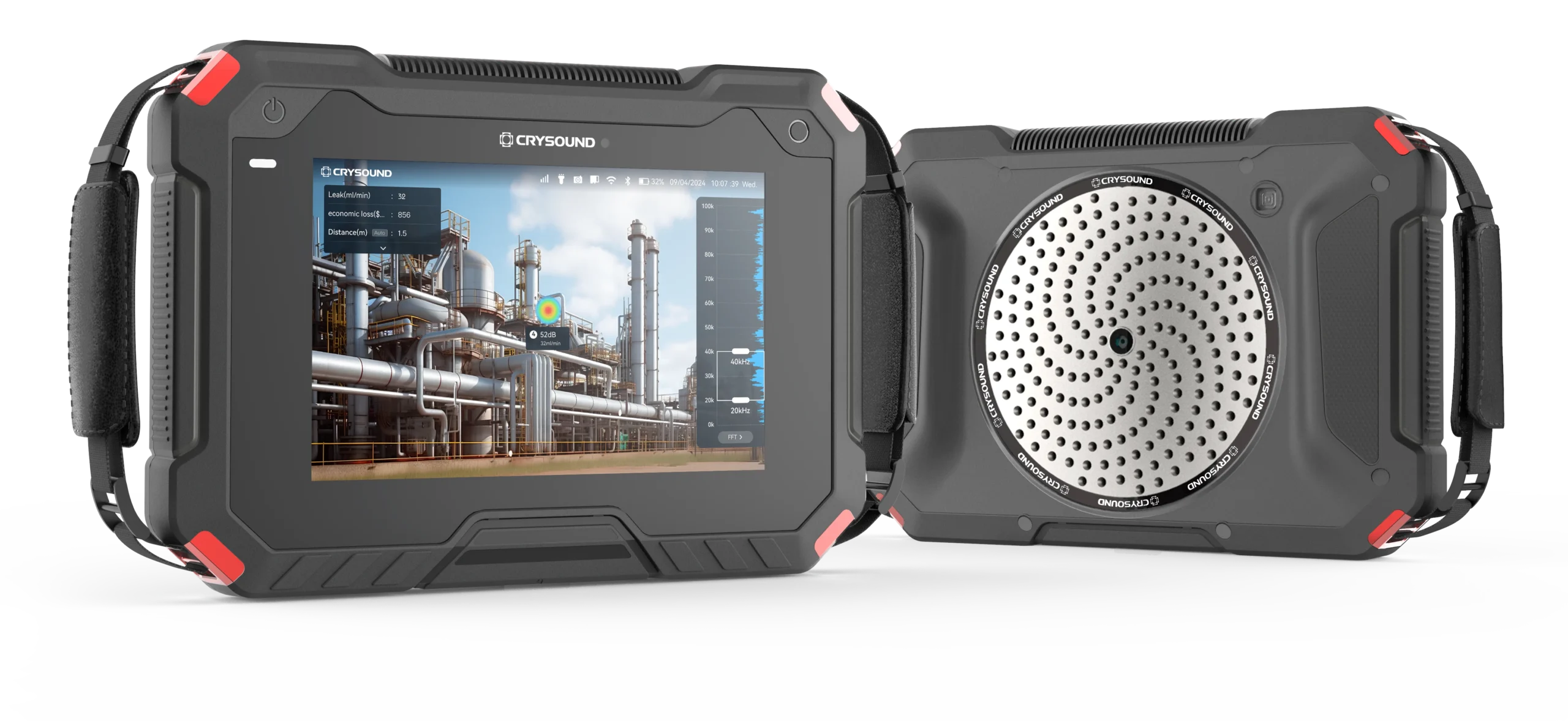
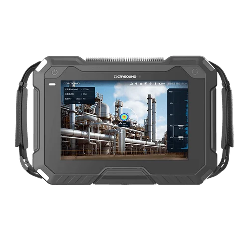
CRY8125 Ex Advanced Acoustic Imaging Camera
Measure Sound Better
Measure Sound Better
At CRYSOUND, precision blends innovation. With over 25 years of expertise in acoustic measurement, we deliver cutting-edge solutions that drive progress from consumer electronics to environmental management. Looking to the future, we are committed to providing world-class acoustic testing equipment while empowering users to be the champions of audio test and detection solutions.
Solutions
Industry leading solutions for accurate acoustic measurements
Gas Leak Detection
CRYSOUND offers a versatile gas leak detection solution for both ordinary and explosion-proof...
Noise and Vibration Test
CRYSOUND conducts noise and vibration tests for diverse environments, encompassing traffic, airport...
Electroacoustic Test
CRYSOUND's electroacoustic test solutions are tailored to assess a wide range of consumer...
Blog
Company News, Case Study

Ways to Connect a DAQ to a PC: Ethernet, USB, WiFi, and PXIe
Before you begin any formal data acquisition work, one critical step is connecting the DAQ front end to the PC. In day‑to‑day engineering, the most common options include USB direct connection, Wi‑Fi wireless, Ethernet, and PXIe. This article introduces these four common connection methods from several angles—how they differ, where each one shines, and their practical limitations—to help you build a deeper, more intuitive understanding of DAQ connectivity. Ethernet Connection An Ethernet connection means the front end joins a local area network (LAN) through its network port, and the PC accesses the device over IP. A typical data path looks like this: Sensor → front‑end sampling → Ethernet transport (TCP/UDP, etc.) → PC/server storage and processing. This topology ranges from very simple to quite complex, for example: Front end ↔ PC (point‑to‑point direct link) Multiple front ends → switch → PC/server (distributed) Figure 1. Ethernet Connection Advantages of Ethernet Connections Flexible topology: single‑node, multi‑node, and distributed setups are all easy to organize; Comfortable distance and cabling: copper Ethernet or fiber makes it easier to deploy across rooms, floors, or even buildings—and routing can be more standardized; Mature infrastructure and strong maintainability: switches, cables, transceivers, fiber, and rack accessories are widely available, and issues are usually easier to locate and troubleshoot; Limitations of Ethernet Connections The network introduces uncertainty—topology, switch performance, port congestion, broadcast storms, and link errors can all cause throughput/latency fluctuations; With multiple devices/nodes, the need for network planning rises quickly: IP addressing, subnetting, whether to use DHCP, routing across subnets, switch cascade depth, etc. As the system grows, things can get messy without a plan. Cable quality, shielding/grounding, routing close to high‑power lines, poor port contact, or switch power instability may show up as packet loss, retransmissions, or speed‑negotiation anomalies. For engineers, Ethernet is straightforward on the test floor: in many setups, a single cable is enough to bring the DAQ front end online with the PC—parameter setup, start/stop, live monitoring, and logging all feel smooth. When the distance grows, you can extend the copper run or switch to fiber to keep transmission stable. In cross‑floor or multi‑room environments—or where noise/safety constraints make it inconvenient to stay near the rig—data can be acquired and monitored from an office or control room over the network. Of course, very long cable runs can be a headache in their own right. SonoDAQ Pro comes standard with two Gigabit LAN ports (GLAN, daisy‑chain capable, supporting 90 W PoE++ power delivery) and also provides a USB‑C port with gigabit‑class throughput, giving users more flexible network‑style connection options. Figure 2. SonoDAQ Rear Panel Wi‑Fi Connection Wi‑Fi DAQ means the acquisition node communicates with a PC or a LAN over a wireless network. Unlike simply “replacing the cable with wireless,” Wi‑Fi DAQ systems typically have two working modes: Real‑time streaming: after sampling, data is sent to the PC over Wi‑Fi in real time; Local buffering/storage: data is first buffered or stored on the front end; Wi‑Fi is used mainly for control, preview, transferring selected segments, or exporting after the run. Two common networking setups are: The DAQ front end joins an on‑site access point (STA mode); The PC creates a hotspot and the DAQ front end connects to it. In short, the front end must support Wi‑Fi, and it must be on the same LAN as the PC. Figure 3. Wi-Fi Connection Advantages of Wi‑Fi Connections No cabling: when wiring is difficult or not allowed, the DAQ can be placed close to the measurement point and controlled over Wi‑Fi; Flexible remote acquisition: by mapping the DAQ’s IP to the public Internet, the PC can access the DAQ by IP address for ultra‑long‑distance remote control. Limitations of Wi‑Fi Connections Uncertainty for sustained high‑volume transfers: available wireless bandwidth can change at any time, so long, continuous acquisitions are more likely to expose packet loss/retransmissions/buffer overflows—the heavier the data load, the more obvious this becomes; Stability depends heavily on the environment: multipath, co‑channel interference, AP congestion, and movement (changing the RF path) can all cause throughput swings and higher latency/jitter, showing up as choppy live plots or occasional disconnect/reconnect events. In real projects, Wi‑Fi is most often used when cabling is inconvenient or prohibited, or when remote/off‑site acquisition is required but running Ethernet is impractical. Engineers can configure parameters remotely, start/stop acquisition, monitor key metrics, or pull specific segments. For larger datasets or long‑duration logging, it’s common to pair Wi‑Fi with front‑end buffering/local storage—Wi‑Fi keeps things visible and controllable, while the front end protects data integrity. USB Connection A USB DAQ device typically means sampling happens in an external front end (with built‑in ADCs, signal conditioning, clocks, etc.). The PC handles configuration, visualization/analysis, and data storage, while USB “moves” the data into the computer. In this relationship, the PC acts as the USB host and the front end acts as the USB device. Figure 4. USB Connection Advantages of USB Connections Low barrier and quick to start: no IP setup and no dependency on network infrastructure—plug it in, install the driver/software, and you can usually start acquiring; Highly portable: an external box plus a laptop is a common combo, well suited to field work, customer sites, and temporary setups; Ubiquitous interface: cables, adapters, mounting clips, and docks are easy to source; Limitations of USB Connections Scalability is generally less “natural” than network/platform approaches. When a system grows from a single front end to multiple front ends and coordinated multi‑point measurements, cabling, device management, and synchronization depend more on the specific implementation; If multiple high‑throughput devices share the same USB controller (DAQ front end, external SSD, camera, etc.), you may see throughput fluctuations, buffer warnings, and occasional stuttering. USB controllers, driver stacks, system load, and power‑management policies vary from PC to PC, so the same device can behave differently on different hosts. Most USB front ends are portable external devices. They often integrate a reasonably complete set of general‑purpose measurement interfaces—analog inputs/outputs, digital I/O, counters/encoders, etc. With a single USB cable, you get both connection and control to the PC for acquisition, display, and storage. As a result, USB is widely used for temporary measurements in the field or at customer sites, rapid R&D bring‑up and debugging, and small‑channel, short‑duration tests. PXIe Interface PXIe is a platform form factor built around a chassis, backplane, and modules. Measurement/instrument modules plug into the chassis and interconnect through the backplane; the chassis then works with a controller or an external link to a PC workstation. Compared with a single external DAQ box, PXIe is more platform‑oriented, modular, and capable of system‑level composition. If a PXIe controller is installed in the chassis, the chassis effectively becomes the host and can run acquisitions independently. Without a PXIe controller, a PXIe chassis is typically not connected to a PC via a standard Ethernet port. Instead, it uses a remote‑control link that essentially “extends the PCIe bus” so an external PC can see the chassis modules as if they were local PCIe devices. In practice, the two most common options are MXI‑Express (a host interface card in the PC plus a remote‑control module in the chassis, linked with a dedicated cable) and Thunderbolt. A typical data path looks like this: Sensor → PXIe module sampling/processing → chassis backplane → controller/link → PC/storage Figure 5. PXIe interface Advantages of PXIe Interface You can populate the chassis with the functional modules you need (analog, digital, bus interfaces, switch matrices, etc.). System capability comes from the “module mix,” and adding or swapping modules later is straightforward; High level of engineering integration: power, cooling, and mechanical form factor feel more like a test platform. In rack/bench systems, cabling, maintenance, and spare‑parts management are easier to standardize; When a test system is expected to evolve—more channels, more functions, module upgrades over time—the platform’s long‑term scalability is a strong advantage. Limitations of PXIe Interface Higher cost and larger footprint: a chassis + module ecosystem is typically a bigger investment than “PC + single card/box,” and it tends to be a fixed installation. Less friendly for mobile/field work: for scenarios that require frequent transport and rapid setup, PXIe’s platform advantages can become a burden; Higher system‑build complexity: it’s more like building a test system, where rack layout, harness management, thermal design, power headroom, and grounding all need to be considered. In practice, SonoDAQ Pro adopts a PCIe‑based modular backplane architecture. Each functional module connects to the main control platform (ARM) through the backplane for high‑speed data uplink/downlink, synchronization, and power distribution. We call this internal interconnect “Trilink.” While enabling modular expansion, SonoDAQ Pro also supports external communication interfaces such as GLAN, Wi‑Fi, and USB‑C, significantly improving deployment flexibility. For a more hands‑on view of how SonoDAQ works over different connection methods (USB / Wi‑Fi / GLAN)—including real usage workflows, representative scenarios, and common configuration checklists—please fill out the Get in touch form below and we’ll reach out shortly.
Bridging the A²B Audio Bus to Measurements
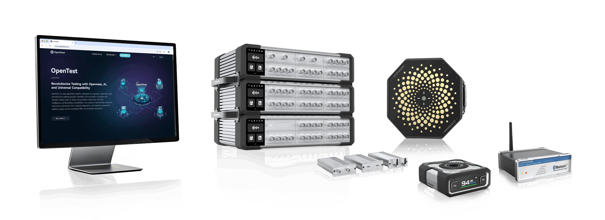
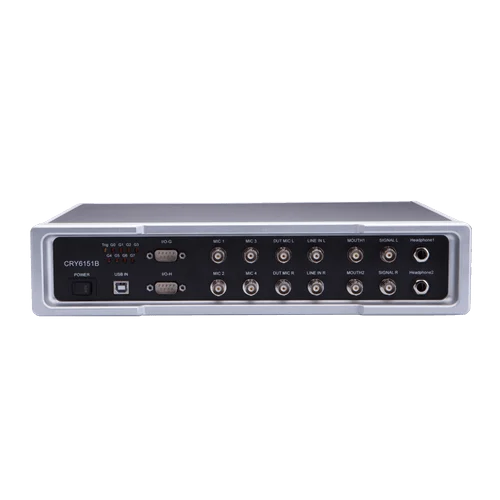
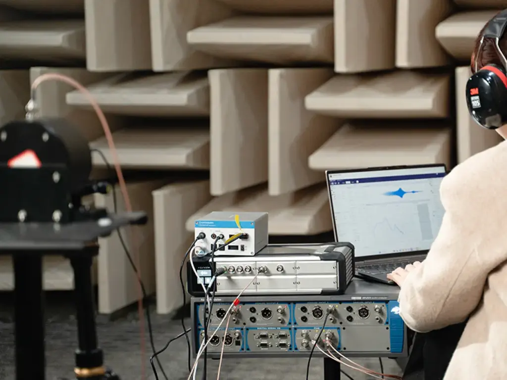
CRY580 A²B Interface is a bidirectional bridge designed to connect the A²B (Automotive Audio Bus) ecosystem with standard test & measurement setups (e.g., SonoDAQ, CRY6151B, Audio Precision). This article explains what makes A²B testing challenging—most analyzers don’t have a native A²B interface—and how CRY580 solves it by encoding/decoding A²B streams and converting them into measurable Analog or S/PDIF outputs, while supporting multi-channel I²S/TDM audio paths for fast, repeatable validation. Faster Automotive Audio Testing with CRY580 One bidirectional A²B bridge for testing: apply an analog/digital test stimulus for A²B amplifier testing, and bring A²B microphone or accelerometer sensor streams out as analog or S/PDIF for measurement. The A²B Audio Bus Is Reshaping In-Vehicle Audio A²B technology enables cost-effective audio data transport over long distances, combining multichannel audio (I²S/TDM), control (I²C), and power delivery over affordable cabling. Bidirectional data transfer at 50 Mbps bandwidth Low and deterministic latency(50 µs) System-level diagnostics Slave nodes can be locally-powered or bus-powered Programmable using ADI's SigmaStudio® GUI Uses cost-effective cables(unshielded twisted pair) The Testing Pain: A²B Adds Performance—And Complexity Traditional audio analyzers do not include A²B interfaces, making it impossible to directly test A²B devices. To perform accurate testing, a dedicated A²B codec is required to decode and convert A²B audio signals into standard analog or digital formats for measurement and analysis. How Bridging to Measurements Works in Practice How A²B Technology and Digital Microphones Enable Superior Performance in Emerging Automotive Applications A²B Microphone A²B Accelerometer A²B Amplifier "Bridging" in practice means converting A²B audio signals into standard analog or digital formats for testing: for A²B amplifier testing, injecting analog/digital stimulus into the A²B bus; and for A²B sensor testing, extracting A²B audio data to analog or S/PDIF for measurement. The CRY580 serves as the ideal bidirectional test bridge, facilitating seamless conversion and measurement in both directions. Introducing CRY580: An A²B Interface Built for Automotive Testing The CRY580 is a versatile A²B interface designed to seamlessly bridge A²B networks with testing equipment. It provides both decoding and encoding capabilities, allowing for the efficient transfer of audio data between A²B devices and standard measurement systems. Whether you're testing A²B microphones, amplifiers, or sensors, the CRY580 enables smooth and reliable testing workflows, ensuring accurate results across a range of automotive audio applications. CRY580 A²B Interface Who Buys CRY580 and What They Test OEM / Tier1 Audio Teams: Integration, debugging, and acceptance testing across A²B networks. A²B Microphone & Mic-Array Suppliers: Sensitivity, frequency response (FR), and phase consistency checks. A²B Amplifier / Audio Processor Suppliers: Amplifier testing with injected stimuli, as well as mapping and performance verification. Test Labs: Standardized A²B measurement processes and delivery. Manufacturing / EOL QC: Repeatable pass/fail testing with faster fault isolation. Typical Test Setups: More Than Just an Interface At CRYSOUND, we provide more than just the CRY580 A²B interface. We offer a full automotive audio testing solution, including audio acquisition cards, microphones and sensors, acoustic sources, custom fixtures, acoustic test boxes, and vibration shakers, delivering a complete and streamlined testing experience. Here’s a description of the testing block diagram, including the use of the latest OpenTest Audio Test & Measurement Software https://opentest.com The CRY580 A²B Interface can be used in conjunction with the Audio Precision. Digital Interface Analog Interface "Performing A²B microphone performance tests (Frequency Response, THD+N, Phase, SNR, AOP) in an anechoic chamber, using the CRY5820 SonoDAQ Pro, CRY580 A²B Interface, and other equipment.” Why CRYSOUND: A Complete Automotive Audio Test Ecosystem The value of end-to-end delivery: reducing system integration time and minimizing coordination costs between multiple suppliers. We cover everything from R&D to production line testing. BOM list of the solution CRY580 bridges A²B to mainstream test & measurement setups in both directions, turning complex in-vehicle audio validation into a faster, repeatable workflow from R&D to end-of-line production. To discuss your use case, system configuration, or a demo, please fill out the Get in touch form below and we’ll reach out shortly.

FFT Analysis with OpenTest
In audio and vibration testing, FFT analysis (Fast Fourier Transform) is one of the tools almost every engineer uses sooner or later: Loudspeaker frequency response Headphone distortion NVH diagnostics Structural resonance troubleshooting Production noise and “mysterious tone” hunting A lot of practical questions are actually asking the same few things: Where is the energy concentrated in frequency? Is it dominated by one tone or a bunch of harmonics? How high is the noise floor? Are there any resonance peaks? FFT is the most universal entry point to answer these questions. This article will help you clarify three things from an engineering perspective: What FFT analysis is How FFT works conceptually How to use FFT correctly and efficiently in practice What Is FFT? In the time domain, a signal is just a waveform changing over time – all components “stacked together” in one trace. You can see it, but it’s hard to tell which frequencies are inside. FFT (Fast Fourier Transform) decomposes a time-domain signal into a sum of sinusoids at different frequencies. In the frequency domain, the signal is represented by frequency + amplitude + phase. In simple terms: Time domain: how the signal moves over time Frequency domain: what frequency components it contains, which are strongest, and how they relate to each other Historically, Fourier’s key idea (early 19th century) was that a complex periodic function can be expressed as a sum of sines and cosines. This evolved into the continuous-time Fourier transform, mapping signals onto a continuous frequency axis. In the computer age, things changed: engineers work with sampled data and typically only have a finite-length record of N samples. That leads to the DFT (Discrete Fourier Transform), which maps N time samples to N discrete frequency bins. FFT (Fast Fourier Transform) is not a different transform. It is a family of algorithms that compute the exact same DFT much more efficiently: Direct DFT: complexity ~ O(N²) FFT: complexity ~ O(N log N) The output X[k] is identical to the DFT result – FFT just gets there far faster by exploiting symmetry and divide-and-conquer. What FFT Is Good at – and What It Isn’t FFT is very good at: Finding deterministic narrowband components Fundamental tones, harmonics, switching frequencies, whistle tones, speed-related lines Looking at broadband distributions Noise floor, 1/f slopes, in-band power, SNR Characterizing system behavior Transfer functions, resonances / anti-resonances, coherence, delay estimation Serving as the foundation of time–frequency analysis STFT, spectrograms, etc. FFT is not good at (or not sufficient on its own for): Strongly non-stationary signals and “instantaneous frequency” For chirps and rapidly changing content, you need STFT, wavelets, or other time–frequency methods, not a single FFT on a long record Separating two extremely close tones below your frequency resolution If the spacing is smaller than your bin resolution (set by N), no algorithm will magically resolve them Turning short data into “long measurements” Zero padding only interpolates the spectrum visually; it does not add new information Before Using FFT: Key Concepts to Get Right To use FFT well, you need to be confident about a few fundamentals: Sampling rate DFT and its interpretation What you actually plot (magnitude, amplitude, power, PSD) Windowing and spectral leakage Averaging Sampling Rate: How High in Frequency You Can See Before FFT, you already made one crucial decision: sampling. A continuous-time signal x(t) is turned into a discrete sequence x[n]=x(n/fs). The sampling rate fsf_sfs determines the highest frequency you can observe without aliasing: the Nyquist frequency, fs/2. If the analog signal contains energy above fs/2, it does not disappear – it folds back into the band below Nyquist as aliasing. Once aliasing happens, FFT cannot “undo” it; the information is irretrievably mixed. In practice, you must use an anti-alias filter before the ADC (or before any resampling) to suppress components above Nyquist. Example: A 900 Hz sine sampled at fs=1 kHz will appear at 100 Hz in the discrete spectrum – a classic aliasing artifact. DFT Computation and Interpretation Given N samples x[0]..x[N−1], the DFT is defined as: The inverse transform (IDFT) reconstructs the time signal: Intuitively, X[k] tells you how strongly the signal correlates with a complex exponential at that bin’s frequency. The magnitude X[k] indicates “how much” of that frequency component exists The phase encodes time alignment relative to other components What Are You Plotting? Magnitude, Amplitude, Power, PSD From one set of FFT results X[k], you can create many different “spectra” that look similar but represent different physical quantities. This is where confusion between tools and platforms often arises. Common variants include: Magnitude spectrum |X[k]| Units depend on normalization (e.g., “V·samples”) Useful for locating peaks, harmonics, and general spectral shape Amplitude spectrum Properly scaled magnitude, in physical units (e.g. V) Appropriate for reading off sinusoid amplitudes and doing calibrated measurements Power spectrum |X[k]|² Again, scaling dependent; often used for power/energy comparisons when conventions are fixed Power Spectral Density (PSD) Sxx(f) Units like V²/Hz or Pa²/Hz Used for noise analysis, band power, and comparisons across different FFT lengths If you want to compare noise levels across different FFT sizes, windows, or tools, use PSD (or amplitude spectral density). Raw |X| or |X|² values are rarely directly comparable. A Concrete Example: Two Tones in Time and Frequency Imagine a signal consisting of two sinusoids at different frequencies. In the time domain, their sum may look like a “wobbly” waveform. In the frequency domain (FFT/PSD), you will see two distinct narrow peaks at the corresponding frequencies. In OpenTest’s FFT analysis, you can visualise both the spectrum and PSD/ASD side by side, making it easy to: Identify tonal components Inspect noise distribution Compare different operating conditions on the same frequency grid Try it yourself: Download the free OpenTest edition and run an FFT on a simple two-tone signal to see both peaks clearly separated. Window Functions and Spectral Leakage: Cleaning Up Spectra In theory, FFT assumes the sampled block contains an integer number of periods and is then repeated periodically. In reality, the record almost never lines up perfectly with an integer number of cycles. When you repeat that block, you get discontinuities at the boundaries, which causes energy to spread into neighboring bins — this is spectral leakage. To reduce leakage, we typically apply a window function to the time record before doing FFT. A window simultaneously affects: Main lobe width Wider main lobe = peaks get broader → it’s harder to separate close tones Side lobe height Lower side lobes = easier to see small peaks near a large one (better dynamic range) Amplitude/energy scaling Windows change the relationship between a pure tone’s true amplitude and the observed peak, as well as the noise floor level Some practical guidelines: Rectangular window Only use when you can ensure coherent sampling (an integer number of periods in the record) and you want the narrowest possible main lobe Hanning (Hann) window A very robust default choice for general acoustics and vibration work Widely used with Welch/PSD methods Hamming Similar to Hann, with slightly different side-lobe behavior, common in communications Blackman / Blackman–Harris Lower side lobes, useful when you need to see small peaks next to big ones, at the cost of a wider main lobe In OpenTest, you can switch between different window functions in the FFT analysis module and immediately see the impact on peak width, side lobes, and noise floor. Averaging: Making Spectra More Stable For noisy or non-stationary signals, a single FFT can look very “spiky” or unstable. By averaging multiple spectra, you obtain a smoother, more repeatable result. Common averaging types include: Linear averaging A simple arithmetic mean of several FFT results Exponential averaging Recent data gets more weight; good for live monitoring when the spectrum should react but not jump wildly Energy (power) averaging Based on power; ensures power-related quantities remain consistent A good averaging configuration strikes a balance between suppressing random fluctuations and preserving genuine changes in the signal. Where Do We Use FFT in Practice? Audio and Acoustics Typical applications include: Finding feedback frequencies, harmonic distortion, and device noise floors Frequency response (transfer function) measurement Room modes / resonance analysis Spectrograms of speech, music, and equipment noise In audio/acoustics, you must be clear about units and conventions: dB SPL, A-weighting, 1/3-octave bands, etc. FFT is the engine; the reporting convention (reference, weighting, bandwidth) must be clearly defined. Vibration and Rotating Machinery Identifying speed-related peaks (1X, 2X, gear mesh frequencies) Structural resonances and mode behavior under different operating conditions Bearing diagnostics, gear whine, imbalance, misalignment For bearing and gearbox analysis, envelope detection/demodulation is often used: Band-pass filter the signal Demodulate and then perform FFT on the envelope to reveal fault frequencies If the rotational speed is changing, a simple FFT will “smear” peaks. In that case, order tracking or synchronous resampling is more appropriate, turning the axis from “frequency” into “order”. Power Electronics and Power Quality Line frequency harmonics (50/60 Hz and multiples), THD, ripple, switching spikes Pre-compliance EMI checks: spectral lines, noise floor, in-band power In power systems, non-coherent sampling is a common issue: if the record length is not an integer number of mains cycles, leakage affects harmonic accuracy. Solutions include synchronous sampling, integer-cycle windows, or specialized harmonic analyzers. RF and Communications (Baseband View) Modulated signal spectra and spectral masks OFDM and multi-carrier spectral analysis, adjacent channel leakage Here, consistency is paramount: Same units Same bandwidth (RBW) Same window, detector, and averaging style FFT itself is straightforward; turning it into comparable power measurements requires tightly defined settings. Imaging and 2D Filtering 2D FFT extends the same idea to images: Edges correspond to high spatial frequencies; smooth areas to low frequencies Low-pass / high-pass filtering, removal of periodic noise, convolution acceleration in the frequency domain The same periodic extension assumption now applies in 2D: discontinuities at image borders produce strong artifacts in the frequency domain. Padding, mirrored borders, or 2D windows are common ways to mitigate this. Turning FFT into an Everyday Engineering Tool From a mathematical standpoint, FFT is not particularly “lightweight”. But in engineering use, the goal is actually simple: See what’s hidden inside the signal more clearly and much faster. When you understand: What FFT really computes How sampling, windowing, scaling, and averaging affect the result When to use spectra vs PSD, and which settings matter for your use case …then FFT stops being an abstract math topic and becomes a practical, everyday tool for acoustics and vibration work – from R&D and validation all the way to production testing. Download and get started now -> or fill out the form below ↓ to schedule a live demo. Explore more features and application stories at www.opentest.com.
Get in touch
Are you seeking more information about CRYSOUND’s solutions or need a demo? Contact us via the form bleow and one of our sales or support engineers will connect with you.
Sound and Vibration Test & Measurement - CRYSOUND
Measure Sound Better
At CRYSOUND, we blend precision with passion. With over 25 years of experience in delivering high-quality acoustic measurement products, we are dedicated to providing advanced solutions that empower users to be the champions of audio test and detection solutions.